This Python 3.11 script trains a simple convolutional neural network (CNN) for the CIFAR-10 (external link)
dataset image classification problem. It's implemented using the PyTorch package and briefly visualizes its performance for various hyperparameter settings.
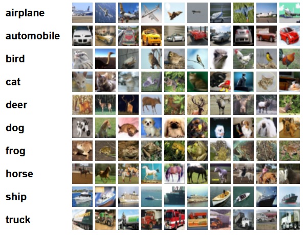
The dataset itself consists of 60000 images of 32x32 pixel size, with each showing some object/animal of a single class. The classes are:
"airplane", "automobile", "bird", "cat", "deer", "dog", "frog", "horse", "ship" and "truck". There are 6000 images for each class and
the data is split into 50000 training and 10000 test images.
The Python files consist of 5 modules for: Preprocessing and loading the data, setting up our CNN class, training the CNN on the data,
visualizing the results and lastly the main module that imports the other modules to execute the functions therein.
While the CNN is very simple in structure, its performance isn't too bad (especially considering the small size of the images),
with an image classification accuracy of about 74% on the testing set, when using the last hyperparameter settings tested in the code.
There would be several ways of further improving the performance of our CNN: More finetuning of the parameters (learning rate,
number of epochs, batch size), adjusting the convolutional or fully connected layers, adding other techniques like dropout
(dropping nodes during training), making the learning rate dynamic (updating it after every epoch) or automatically stopping the
training, once the test performance isn't improving anymore for several epochs.
However, all those methods are omitted here, to keep it simple.
Download (Python 3.11 script as .zip).
"""
    Knowledgedump.org - Image Classification - image_classification
    This script trains a simple CNN model for the CIFAR-10 dataset and briefly analyzes its performance.
    (CIFAR-10 dataset from "Learning Multiple Layers of Features from Tiny Images", Alex Krizhevsky, 2009)
    The individual steps are carried out in the respective modules, with the names being self-explanatory for their function:
        - preprocess_images.py - load + preprocess data for training
        - define_model.py - set up CNN model,
        - train_model.py - train the model on data and evaluate at each step.
        - visualize_results.py - function for visualizing the results with matplotlib.

    Required packages: torch, torchvision, numpy, matplotlib
"""

from preprocess_images import load_and_preprocess_cifar10
from define_model import SimpleCNN
from train_model import train_model
from visualize_results import plot_results

# Train and evaluate model with different parameters:
if __name__ == "__main__":

    # Load and preprocess CIFAR-10 dataset with batch_size=32.
    trainloader, testloader = load_and_preprocess_cifar10(batch_size=32)

    for epo, lrn in zip([10, 10, 20, 20], [0.001, 0.0005, 0.001, 0.0005]):
        # Initialize our "SimpleCNN" model.
        model = SimpleCNN()

        # Train the model with the parameters
        perf_res = train_model(model, trainloader, testloader, epochs=epo, learning_rate=lrn, device=None)

        # Visualize the performance results.
        plot_results(*perf_res)
"""
    Knowledgedump.org - Image Classification - preprocess_images
    Loading and preprocessing the images from CIFAR-10 dataset.

    Required packages: torch, torchvision, numpy, matplotlib
"""

import torch
import torchvision
import numpy as np
import matplotlib.pyplot as pypl
import os, sys


# Function for preparing the data, returning the DataLoaders for the training and testing dataset.
# Default batch size set to 32 by default as solid middle ground.

def load_and_preprocess_cifar10(batch_size=32):
    """
        When loading the dataset from the library torchvision, the images are pillow class objects, with each pixel in
        the 32x32 images being assigned an RGB value, i.e. [0,255]x[0,255]x[0,255]. For potentially faster/more stable
        training later on, we rescale this to values [-1,1]x[-1,1]x[-1,1].
        The transformations we apply can be directly fed into the torchvision.datasets.CIFAR10 class via the
        "transform" parameter, which takes a function with input of a PIL object and outputs a transformed version of it.
    """
    # Compose the transformation of the PIL object into one function.
    trafo = torchvision.transforms.Compose([
        # Transform PIL object to a torch.FloatTensor object of shape C x H x W, where C is the channel count (3 here)
        # and H x W are the image dimensions. The individual RGB values between [0,255] are automatically rescaled to [0,1].
        torchvision.transforms.ToTensor(),
        # Next, rescale to zero centered values in the range [-1,1]. An alternative could be to omit this step and
        # keep the [0,1] values or calculate the means and standard deviation of each channel value, in order to standardize
        # them to a mean of 0 and a standard deviation of 1 (z-score normalization).
        torchvision.transforms.Normalize((0.5, 0.5, 0.5), (0.5, 0.5, 0.5))
    ])

    # Load the CIFAR-10 dataset. Download the dataset to the directory of the script calling this module (if not already present).
    # Apply transformations to get rescaled torch.FloatTensor objects for training and testing set.
    destination_dir = os.path.join(os.path.dirname(os.path.abspath(sys.argv[0])), "data")
    trainset = torchvision.datasets.CIFAR10(root=destination_dir, train=True, download=True, transform=trafo)
    testset = torchvision.datasets.CIFAR10(root=destination_dir, train=False, download=True, transform=trafo)

    # Create training and testing DataLoaders for batch processing.
    trainloader = torch.utils.data.DataLoader(trainset, batch_size=batch_size, shuffle=True)
    testloader = torch.utils.data.DataLoader(testset, batch_size=batch_size, shuffle=False)

    return trainloader, testloader


"""
    Function for displaying the loaded images of a batch with matplotlib, to get a feeling for the data.
    This displays a batch of images in a grid and names their respective content on top (left to right).
    Input parameters:
        - images: Batch of images,
        - labels: Corresponding labels for the images (0,1,...,9),
        - classes: List of class names (airplane, automobile etc.).
"""

def show_images(images, labels, classes, batch_size):
    # Convert the tensor images to a grid.
    img_grid = torchvision.utils.make_grid(images)
    # Create a numpy array from the data. To visualize it with matplotlib, we have to rescale the [-1,1] values back to [0,1].
    np_img = img_grid.numpy()
    np_img = (np_img + 1) / 2

    # Since the tensor objects are of shape C x H x W and we want H x W x C for displaying with pyplot,
    # transpose the array prior.
    pypl.imshow(np.transpose(np_img, (1, 2, 0)))
    # Add title that describes the content of each image in the grid.
    pypl.title(" ".join([classes[labels[j]] for j in range(batch_size)]))
    pypl.show()


if __name__ == "__main__":
    # Load and preprocess CIFAR-10 dataset with default batch size of 32.
    trainloader, testloader = load_and_preprocess_cifar10()

    # Output number of batches and image shapes to verify the loaded data.
    print(f"Number of training batches: {len(trainloader)}")
    print(f"Number of testing batches: {len(testloader)}")

    # Define CIFAR-10 class names.
    classes = ["airplane", "automobile", "bird", "cat", "deer", "dog", "frog", "horse", "ship", "truck"]

    # Set up iterator on DataLoader of training set.
    dataiter = iter(trainloader)

    # Show 3 batches of training sets.
    for _ in range(3):
        images, labels = next(dataiter)
        show_images(images, labels, classes, batch_size=trainloader.batch_size)
"""
    Knowledgedump.org - Image Classification - define_model
    Defining a simple Convolutional Neural Network (CNN) model class for image classification.
    We use three convolutional layers, each followed by max-pooling and lastly flattening to the fully connected layer.

    Required packages: torch
"""

import torch


class SimpleCNN(torch.nn.Module):
    def __init__(self):

        # Call constructor of PyTorch CNN model class nn.Module .
        super(SimpleCNN, self).__init__()

        # Convolutional layer 1:
        # - 3 input channels (RGB images), 32 output channels (feature maps)
        # - Kernel size of 3x3 with padding=1 to maintain image dimensions (32x32)
        # - used to catch low-level features
        self.conv1 = torch.nn.Conv2d(3, 32, kernel_size=3, padding=1)

        # Convolutional layer 2:
        # - 32 input channels, 64 output channels
        # - used to capture mid-level features
        self.conv2 = torch.nn.Conv2d(32, 64, kernel_size=3, padding=1)

        # Convolutional layer 3:
        # - 64 input channels, 128 output channels
        # - for high-level features
        self.conv3 = torch.nn.Conv2d(64, 128, kernel_size=3, padding=1)

        # Max pooling layer:
        # - Reduces the dimensions of the feature maps for lower computational complexity.
        # - We use a 2x2 kernel with a stride of 2, which reduces the height and width of the image by half.
        self.pool = torch.nn.MaxPool2d(kernel_size=2, stride=2, padding=0)

        # Fully connected layer 1:
        # - After the convolutional layers, we flatten the feature maps into a 1D tensor for the fully connected layers.
        # - The size of the flattened tensor after passing through three convolutional layers and pooling is 128 * 4 * 4,
        #   which is compressed from 2048 to 512 neurons for reduced model complexity.
        self.fc1 = torch.nn.Linear(128 * 4 * 4, 512)

        # Fully connected layer 2 (output layer):
        # - This layer maps the 512 features from the previous layer to 10 output values.
        # - Each of the 10 output values corresponds to the probability of one of the CIFAR-10 classes.
        # - A softmax function will be used at the end of the forward pass to convert the raw outputs (logits) to probabilities.
        self.fc2 = torch.nn.Linear(512, 10)

        # ReLU (Rectified Linear Unit) activation function:
        # - A non-linear activation function applied after each convolutional and fully connected layer.
        # - Helps introduce non-linearity into the model and allows it to learn more complex patterns (faster training).
        # - Function is given by max(0,x).
        self.relu = torch.nn.ReLU()

        # Softmax function (at the end of the forward pass):
        # - The softmax function is applied after the final fully connected layer to convert logits into
        #   class probabilities for each input image.
        self.softmax = torch.nn.Softmax(dim=1)


    """
        Define the forward pass function of the model, where input tensor "inp" sequentially passes through all the layers.
        - input tensor has dimension of batch_size x 3 x 32 x 32 here.
        - output tensor has dimension batch_size x 10, containing the probabilities for each class.
    """

    def forward(self, inp):
        # Pass through the first convolutional layer and apply ReLU activation function.
        inp = self.relu(self.conv1(inp))
        # Apply max-pooling to reduce the height x width dimensions after conv1.
        inp = self.pool(inp)

        # Pass through the second convolutional layer.
        inp = self.relu(self.conv2(inp))
        inp = self.pool(inp)

        # Pass through the third convolutional layer.
        inp = self.relu(self.conv3(inp))
        inp = self.pool(inp)

        # Flatten the output from the convolutional layers into a 1D tensor
        # The output size after pooling is (B x 128 x 4 x 4), and is flattened to (B x 128*4*4).
        inp = inp.view(-1, 128 * 4 * 4)

        # Pass through the first fully connected layer and apply ReLU activation function.
        inp = self.relu(self.fc1(inp))

        # Pass through the second fully connected layer (output layer).
        inp = self.fc2(inp)
        # Apply softmax to the output to get the class probabilities.
        inp = self.softmax(inp)

        return inp
"""
Knowledgedump.org - Image Classification - train_model
Train a Convolutional Neural Network (CNN) model for image classification.
We use a cross-entropy loss function, epoch number of 10 and Adam as optimizer here, with learning rate 0.001.
(Might have to fine-tune these after testing)
Required packages: torch
"""
import torch
import time
"""
Function to train the model with CIFAR-10 data.
Inputs:
- CNN model (object of torch.nn.Module class), i.e. the model to be trained here.
- DataLoaders for training and testing data.
- Number of epochs to train the model (default of 10 here).
- Learning rate for the optimizer (default is 0.001 here).
- Device to train the model on - torch.device("cpu") for CPU or None for GPU (if available).
Returns:
- Epoch loss and accuracy % values for visualization afterwards.
"""
def train_model(model, trainloader, testloader, epochs=10, learning_rate=0.001, device=None):
# Set device to CPU or GPU, depending on availability/setting.
if device == None:
device = torch.device("cuda" if torch.cuda.is_available() else "cpu")
# Print the parameters used and whether CPU (False) or GPU is used (True):
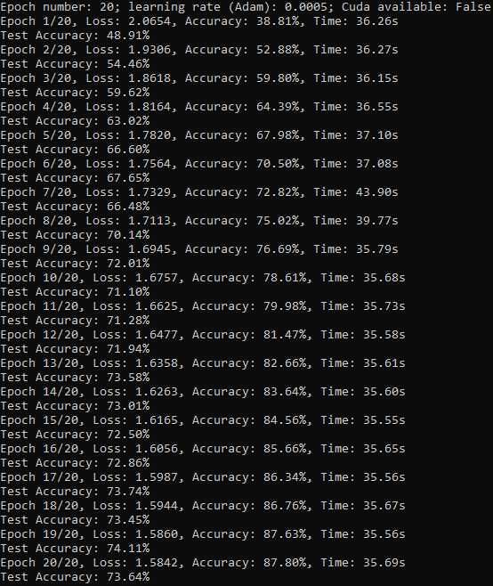
print(f"Epoch number: {epochs}; learning rate (Adam): {learning_rate}; Cuda available: {torch.cuda.is_available()}")
# Initialize lists to store loss and accuracy for visualization
train_epoch_losses = []
train_epoch_accuracies = []
test_epoch_accuracies = []
# Move the model to the selected device (GPU or CPU).
model.to(device)
# Set the optimizer as Adam with respective learning rate.
optimizer = torch.optim.Adam(model.parameters(), lr=learning_rate)
# Use cross-entropy loss function for the image classification problem.
loss_fct = torch.nn.CrossEntropyLoss()
# Loop through the epochs to train the model:
for epoch in range(epochs):
# Set model to training mode.
model.train()
# Variable to accumulate the loss for this epoch.
current_loss = 0.0
# Initialize Counter for correct predictions.
correct_pred = 0
# Total number of images processed.
images_processed = 0
# Record the start time for the epoch.
start_time = time.time()
# Loop through the batches in the training data:
for inputs, labels in trainloader:
# Move the inputs and labels to the selected device (GPU/CPU)
inputs, labels = inputs.to(device), labels.to(device)
# Set gradients from the previous step to zero.
optimizer.zero_grad()
# Perform the forward pass, i.e. compute predicted outputs.
outputs = model(inputs)
# Calculate the loss.
loss = loss_fct(outputs, labels)
# Perform backpropagation (compute gradients).
loss.backward()
# Update the model's parameters, using the optimizer.
optimizer.step()
# Accumulate the loss for this batch.
current_loss += loss.item()
# Get the predicted class labels (highest predicted probability).
_, predicted = torch.max(outputs.data, 1)
# Update correct predictions count.
images_processed += labels.size(0)
correct_pred += (predicted == labels).sum().item()
# Calculate average loss and accuracy in % for this epoch.
epoch_loss = current_loss / len(trainloader)
epoch_acc = 100 * correct_pred / images_processed
epoch_time = time.time() - start_time
# Append the performance values to the output lists:
train_epoch_losses.append(epoch_loss)
train_epoch_accuracies.append(epoch_acc)
# Print out statistics for the current epoch.
print(f"Epoch {epoch + 1}/{epochs}, Loss: {epoch_loss:.4f}, Accuracy: {epoch_acc:.2f}%, Time: {epoch_time:.2f}s")
# Evaluate the model after each epoch, to track progress.
test_epoch_accuracies.append(evaluate_model(model, testloader, device))
return [train_epoch_losses, train_epoch_accuracies, test_epoch_accuracies]
"""
Function to evaluate the trained model on the test set.
Inputs:
- model (torch.nn.Module object) to train.
- DataLoader for test data.
- Device to evaluate the model on (torch.device("cpu") or torch.device("cuda")).
"""
def evaluate_model(model, testloader, device):
# Set the model to evaluation mode (normally used to disable dropouts and batch normalization, which aren't applied here).
model.eval()
# Initialize Counters for correct predictions and total number of processed images.
correct_pred = 0
images_processed = 0
# Disable gradient computation for evaluation (faster and uses less memory)
with torch.no_grad():
# Loop through the test set:
for inputs, labels in testloader:
# Move inputs and labels to the selected device
inputs, labels = inputs.to(device), labels.to(device)
# Perform the forward pass (compute predicted outputs).
outputs = model(inputs)
# Get the predicted class labels.
_, predicted = torch.max(outputs.data, 1)
# Update correct predictions count.
images_processed += labels.size(0)
correct_pred += (predicted == labels).sum().item()
# Calculate the accuracy on the test set in %.
accuracy = 100 * correct_pred / images_processed
print(f"Test Accuracy: {accuracy:.2f}%")
return accuracy
"""
    Knowledgedump.org - Image Classification - visualize_results
    Function for visualizing results after training and testing the CNN model on CIFAR-10 image classification.

    Required packages: matplotlib
"""

import matplotlib.pyplot as pypl

# Input: Lists of training loss values and accuracy % for both the training and testing set.
def plot_results(train_losses, train_accuracies, test_accuracies):
    pypl.figure(figsize=(12, 4))

    # Plot training loss:
    pypl.subplot(1, 2, 1)
    pypl.plot(train_losses, label='Train Loss')
    pypl.title('Training Loss over Epochs')
    pypl.xlabel('Epoch')
    pypl.ylabel('Loss')
    pypl.legend()

    # Plot training and testing accuracy:
    pypl.subplot(1, 2, 2)
    pypl.plot(train_accuracies, label='Train Accuracy')
    pypl.plot(test_accuracies, label='Test Accuracy')
    pypl.title('Training and Test Accuracy over Epochs')
    pypl.xlabel('Epoch')
    pypl.ylabel('Accuracy (%)')
    pypl.legend()

    pypl.tight_layout()
    pypl.show()
Console output (for epochs=10, learning rate=0.001): ---> Learning rate too high.
Visualization:
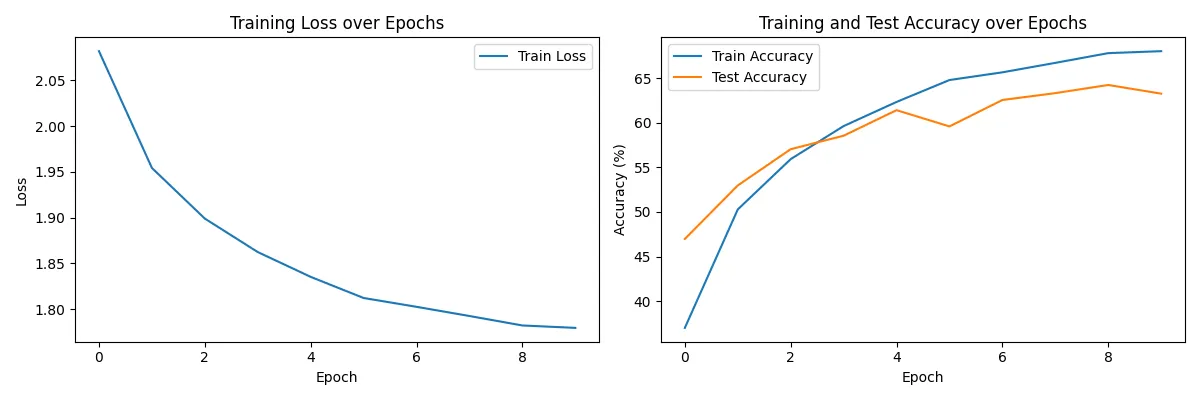
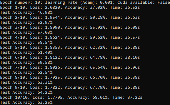
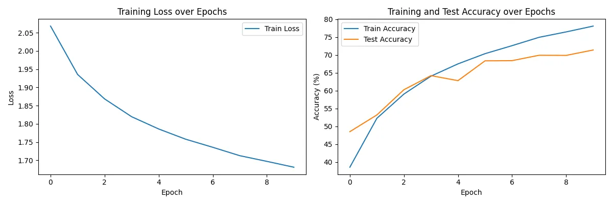
Console output (for epochs=10, learning rate=0.0005): ---> Could use more epochs, might have to lower learning rate more.
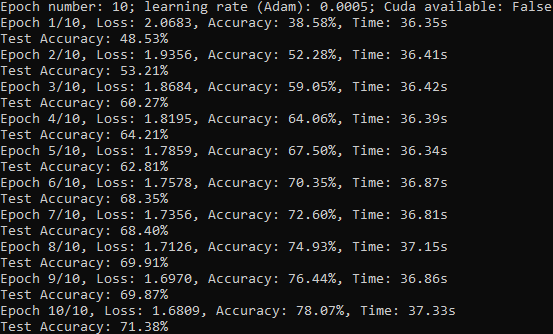
Visualization:
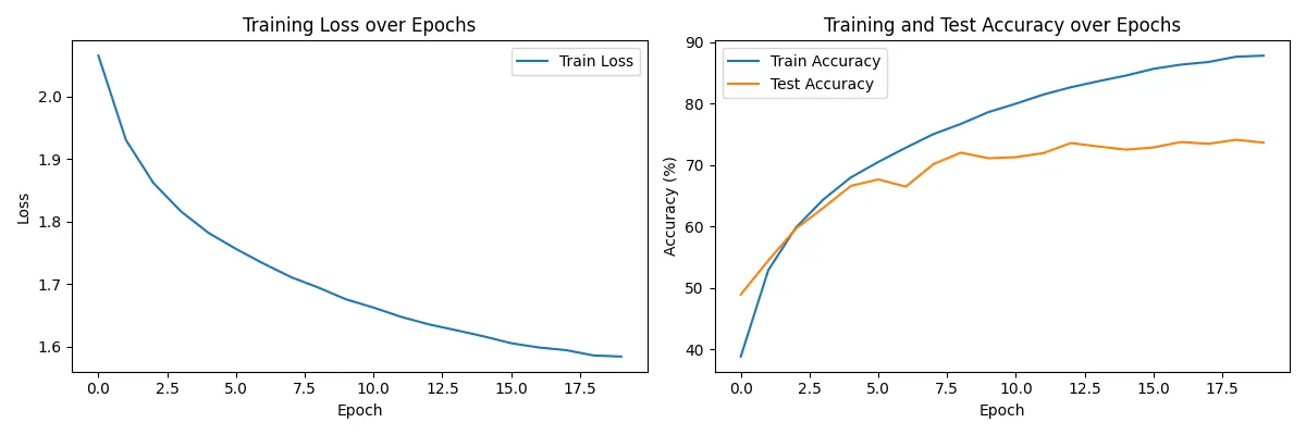
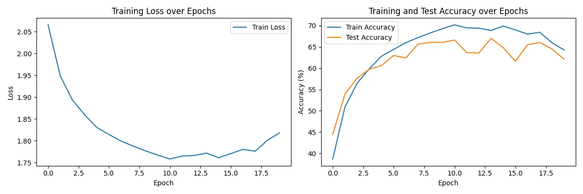
Console output (for epochs=20, learning rate=0.001): ---> Very bad overfitting.
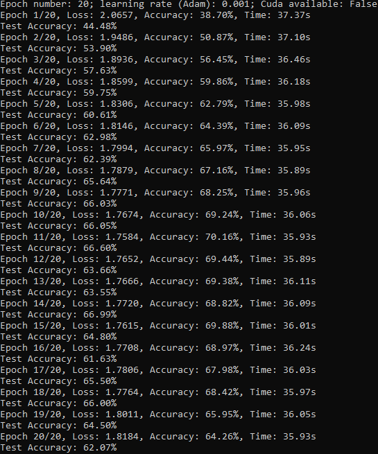
Visualization:
Console output (for epochs=20, learning rate=0.0005): ---> Best combination here. Might be further improved by dynamic lowering of learning rate etc..
Visualization: